Unit IX: Graph (7 Hrs.)
Data Structures & Algorithms — Complete Detailed Chapter Notes
Every topic includes: detailed concept · labeled graph diagrams · pseudocode · step-form algorithm · 2–3 fully-solved traced examples · clean Java code · complexity. Ends with fully-answered important questions (2 / 6 / 10 marks).
Table of Contents
- Introduction
- Graph Terminology
- Types of Graphs
- Graph Representation
- Graph Traversal
- Spanning Tree & Minimum Spanning Tree
- Shortest Path Problem — Dijkstra's Algorithm
- Applications of Graph
- Important Questions with Full Answers
9.1 Introduction
A graph is a non-linear data structure made up of a finite set of vertices (nodes) and a set of edges (links) that connect pairs of vertices. Formally, a graph is written as:
G = (V, E) — where V is the set of vertices and E is the set of edges.
Unlike a tree, a graph:
- may contain cycles (a path that returns to its start),
- need not be connected,
- has no fixed root or parent–child hierarchy, and
- allows a vertex to be connected to any number of other vertices.
Graphs are used to model relationships and networks — road maps, social networks, computer networks, the web, flight routes, and dependencies between tasks. Because of this flexibility, graphs are one of the most important structures in computer science.
Example graph: V = {A, B, C, D} and E = {(A,B), (A,C), (B,C), (C,D)} describes four vertices connected by four edges.
9.2 Graph Terminology
| Term | Definition |
|---|---|
| Vertex (Node) | A fundamental point/entity of the graph. |
| Edge (Arc) | A connection between two vertices. |
| Adjacent vertices | Two vertices joined directly by an edge. |
| Incident edge | An edge is incident on the two vertices it connects. |
| Degree | Number of edges connected to a vertex. |
| In-degree / Out-degree | (Directed graph) number of edges coming into / going out of a vertex. |
| Path | A sequence of vertices connected by edges. |
| Cycle | A path that begins and ends at the same vertex. |
| Loop (self-loop) | An edge from a vertex to itself. |
| Weighted edge | An edge carrying a numeric value (cost, distance, time). |
| Connected graph | A graph in which there is a path between every pair of vertices. |
| Complete graph | Every vertex is directly connected to every other vertex. |
| Subgraph | A graph formed from a subset of the vertices and edges of another graph. |
| Spanning tree | A connected, acyclic subgraph that includes all vertices with exactly V−1 edges. |
9.3 Types of Graphs
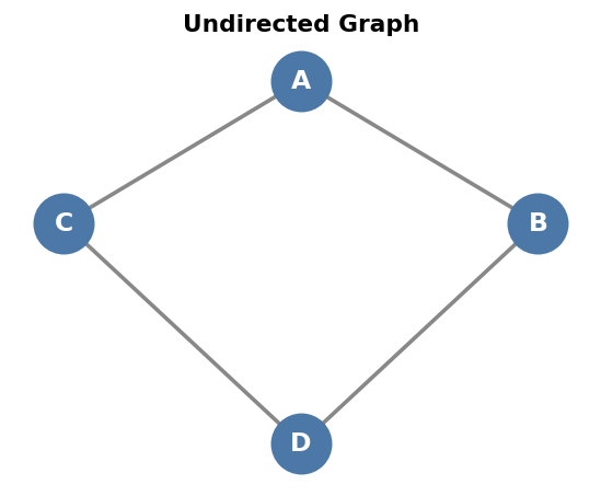
Undirected Graph
Edges have no direction — an edge (A, B) allows movement both ways (A→B and B→A). The relationship is mutual, e.g., friendship on Facebook.
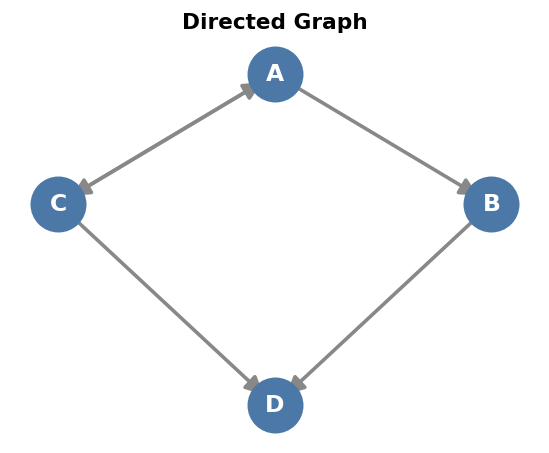
Directed Graph (Digraph)
Edges have a direction shown by arrows — an edge A→B allows movement from A to B only, not necessarily back. Example: "follows" on Twitter, or one-way roads. Each vertex has an in-degree and an out-degree.
Other important types
- Weighted graph: every edge has a weight (used in shortest-path and MST problems).
- Unweighted graph: edges have no weight.
- Cyclic / Acyclic graph: contains a cycle / contains none. A DAG is a Directed Acyclic Graph.
- Connected / Disconnected graph.
| Feature | Undirected Graph | Directed Graph |
|---|---|---|
| Edge direction | None (two-way) | One-way (arrow) |
| Edge notation | (A,B) = (B,A) | (A,B) ≠ (B,A) |
| Degree | Single degree | In-degree & out-degree |
| Example | Friendship network | Web page links, one-way roads |
9.4 Graph Representation
A graph can be stored in memory in two main ways. Consider this sample undirected graph with vertices {0,1,2,3} and edges {0-1, 0-2, 1-2, 2-3}:
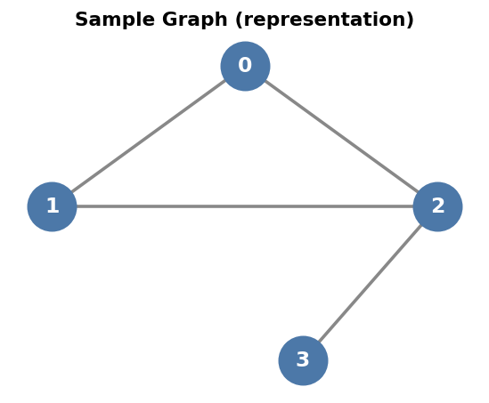
1. Adjacency Matrix
A 2-D array A[n][n] where A[i][j] = 1 if there is an edge between vertex i and vertex j, otherwise 0. (For a weighted graph, store the weight instead of 1.) For an undirected graph, the matrix is symmetric.
| 0 | 1 | 2 | 3 | |
|---|---|---|---|---|
| 0 | 0 | 1 | 1 | 0 |
| 1 | 1 | 0 | 1 | 0 |
| 2 | 1 | 1 | 0 | 1 |
| 3 | 0 | 0 | 1 | 0 |
- Space: O(V²) · Edge lookup: O(1) · Good for dense graphs; wasteful for sparse graphs.
2. Adjacency List
An array (or list) of lists; each vertex keeps a list of its neighbours.
0 → [1, 2]
1 → [0, 2]
2 → [0, 1, 3]
3 → [2]
- Space: O(V + E) · Edge lookup: O(degree) · Good for sparse graphs (most real-world graphs).
| Feature | Adjacency Matrix | Adjacency List |
|---|---|---|
| Space | O(V²) | O(V + E) |
| Check edge (i,j) | O(1) | O(degree) |
| Best for | Dense graphs | Sparse graphs |
| Iterate neighbours | O(V) | O(degree) |
Java — Adjacency List representation
import java.util.*;

public class GraphRepresentation {
    int V;
    List<List<Integer>> adj;

    GraphRepresentation(int V) {
        this.V = V;
        adj = new ArrayList<>();
        for (int i = 0; i < V; i++) adj.add(new ArrayList<>());
    }

    void addEdge(int u, int v) {   // undirected
        adj.get(u).add(v);
        adj.get(v).add(u);
    }

    void print() {
        for (int i = 0; i < V; i++)
            System.out.println(i + " -> " + adj.get(i));
    }

    public static void main(String[] args) {
        GraphRepresentation g = new GraphRepresentation(4);
        g.addEdge(0, 1); g.addEdge(0, 2); g.addEdge(1, 2); g.addEdge(2, 3);
        g.print();
    }
}
9.5 Graph Traversal
Graph traversal means visiting all the vertices of a graph in a systematic order. Because graphs can contain cycles, every traversal uses a visited[] array to make sure no vertex is processed twice (otherwise the algorithm could loop forever). The two standard traversals are BFS (level by level) and DFS (as deep as possible first).
9.5.1 Breadth-First Search (BFS)
Concept (detailed)
BFS explores the graph level by level. Starting from a source vertex, it first visits all its immediate neighbours, then all of their unvisited neighbours, and so on — spreading outward like ripples in water. BFS uses a queue (FIFO) to remember which vertices to visit next. BFS also finds the shortest path (fewest edges) from the source in an unweighted graph.
Pseudocode
procedure BFS(start)
    create empty queue Q
    mark start as visited
    enqueue start into Q
    while Q is not empty do
        v ← dequeue(Q)
        visit v
        for each neighbour u of v do
            if u is not visited then
                mark u as visited
                enqueue u into Q
            end if
        end for
    end while
end procedure
Algorithm (step form)
- Mark the start vertex as visited and put it in the queue.
- Remove a vertex from the front of the queue and process (visit) it.
- For each unvisited neighbour, mark it visited and add it to the queue.
- Repeat steps 2–3 until the queue is empty.
Example 1 — BFS on Graph G1 starting from vertex 0
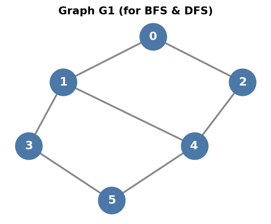
Adjacency: 0→[1,2] · 1→[0,3,4] · 2→[0,4] · 3→[1,5] · 4→[1,2,5] · 5→[3,4]
| Step | Dequeued | Neighbours added | Queue (front→rear) | Visited/Output |
|---|---|---|---|---|
| start | — | — | [0] | 0 |
| 1 | 0 | 1, 2 | [1, 2] | 0 1 2 |
| 2 | 1 | 3, 4 | [2, 3, 4] | 0 1 2 3 4 |
| 3 | 2 | (4 already) | [3, 4] | 0 1 2 3 4 |
| 4 | 3 | 5 | [4, 5] | 0 1 2 3 4 5 |
| 5 | 4 | (all visited) | [5] | 0 1 2 3 4 5 |
| 6 | 5 | (all visited) | [] | 0 1 2 3 4 5 |
BFS traversal order: 0 → 1 → 2 → 3 → 4 → 5
Example 2 — BFS on Graph G2 starting from vertex A
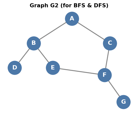
Adjacency: A→[B,C] · B→[A,D,E] · C→[A,F] · D→[B] · E→[B,F] · F→[C,E,G] · G→[F]
| Step | Dequeued | Neighbours added | Queue | Output |
|---|---|---|---|---|
| start | — | — | [A] | A |
| 1 | A | B, C | [B, C] | A B C |
| 2 | B | D, E | [C, D, E] | A B C D E |
| 3 | C | F | [D, E, F] | A B C D E F |
| 4 | D | — | [E, F] | A B C D E F |
| 5 | E | (F already) | [F] | A B C D E F |
| 6 | F | G | [G] | A B C D E F G |
| 7 | G | — | [] | A B C D E F G |
BFS traversal order: A → B → C → D → E → F → G
Java Code
import java.util.*;

public class BFSTraversal {
    static void bfs(List<List<Integer>> adj, int start, int V) {
        boolean[] visited = new boolean[V];
        Queue<Integer> queue = new LinkedList<>();
        visited[start] = true;
        queue.add(start);

        while (!queue.isEmpty()) {
            int v = queue.poll();          // remove from front
            System.out.print(v + " ");     // visit
            for (int u : adj.get(v)) {
                if (!visited[u]) {
                    visited[u] = true;
                    queue.add(u);          // add unvisited neighbour
                }
            }
        }
    }

    public static void main(String[] args) {
        int V = 6;
        List<List<Integer>> adj = new ArrayList<>();
        for (int i = 0; i < V; i++) adj.add(new ArrayList<>());
        int[][] edges = {{0,1},{0,2},{1,3},{1,4},{2,4},{3,5},{4,5}};
        for (int[] e : edges) { adj.get(e[0]).add(e[1]); adj.get(e[1]).add(e[0]); }

        bfs(adj, 0, V);   // 0 1 2 3 4 5
    }
}
Complexity: Time O(V + E) (adjacency list); Space O(V) for the queue and visited array.
9.5.2 Depth-First Search (DFS)
Concept (detailed)
DFS explores the graph by going as deep as possible along one branch before backtracking. Starting from a source, it visits a neighbour, then that neighbour's neighbour, and so on until it reaches a vertex with no unvisited neighbours; then it backtracks to the previous vertex and tries another branch. DFS uses a stack — either explicitly, or implicitly through recursion (the function call stack).
Pseudocode (recursive)
procedure DFS(v)
    mark v as visited
    visit v
    for each neighbour u of v do
        if u is not visited then
            DFS(u)
        end if
    end for
end procedure
Algorithm (step form)
- Mark the current vertex as visited and process it.
- Pick an unvisited neighbour and recursively apply DFS to it.
- If a vertex has no unvisited neighbours, backtrack to the previous vertex.
- Continue until all reachable vertices have been visited.
Example 1 — DFS on Graph G1 starting from vertex 0
(Same graph G1; adjacency 0→[1,2], 1→[0,3,4], 3→[1,5], 5→[3,4], 4→[1,2,5], 2→[0,4].)
| Step | Action | Path (stack) | Output |
|---|---|---|---|
| 1 | visit 0, go to 1 | 0 | 0 |
| 2 | visit 1, go to 3 | 0-1 | 0 1 |
| 3 | visit 3, go to 5 | 0-1-3 | 0 1 3 |
| 4 | visit 5, go to 4 | 0-1-3-5 | 0 1 3 5 |
| 5 | visit 4, go to 2 | 0-1-3-5-4 | 0 1 3 5 4 |
| 6 | visit 2 (neighbours visited) → backtrack all | 0-1-3-5-4-2 | 0 1 3 5 4 2 |
DFS traversal order: 0 → 1 → 3 → 5 → 4 → 2
Example 2 — DFS on Graph G2 starting from vertex A
(Adjacency A→[B,C], B→[A,D,E], D→[B], E→[B,F], F→[C,E,G], C→[A,F], G→[F].)
| Step | Action | Output so far |
|---|---|---|
| 1 | visit A → go B | A |
| 2 | visit B → go D | A B |
| 3 | visit D (only B, visited) → backtrack to B | A B D |
| 4 | from B → go E | A B D E |
| 5 | visit E → go F | A B D E F |
| 6 | visit F → go C | A B D E F |
| 7 | visit C (A,F visited) → backtrack to F | A B D E F C |
| 8 | from F → go G | A B D E F C G |
| 9 | visit G → backtrack (all done) | A B D E F C G |
DFS traversal order: A → B → D → E → F → C → G
Java Code (recursive + iterative)
import java.util.*;

public class DFSTraversal {

    // Recursive DFS
    static void dfs(List<List<Integer>> adj, int v, boolean[] visited) {
        visited[v] = true;
        System.out.print(v + " ");
        for (int u : adj.get(v))
            if (!visited[u]) dfs(adj, u, visited);
    }

    // Iterative DFS using an explicit stack
    static void dfsIterative(List<List<Integer>> adj, int start, int V) {
        boolean[] visited = new boolean[V];
        Deque<Integer> stack = new ArrayDeque<>();
        stack.push(start);
        while (!stack.isEmpty()) {
            int v = stack.pop();
            if (!visited[v]) {
                visited[v] = true;
                System.out.print(v + " ");
                for (int u : adj.get(v)) if (!visited[u]) stack.push(u);
            }
        }
    }

    public static void main(String[] args) {
        int V = 6;
        List<List<Integer>> adj = new ArrayList<>();
        for (int i = 0; i < V; i++) adj.add(new ArrayList<>());
        int[][] edges = {{0,1},{0,2},{1,3},{1,4},{2,4},{3,5},{4,5}};
        for (int[] e : edges) { adj.get(e[0]).add(e[1]); adj.get(e[1]).add(e[0]); }

        dfs(adj, 0, new boolean[V]);   // 0 1 3 5 4 2
    }
}
Complexity: Time O(V + E); Space O(V) (recursion/stack + visited).
BFS vs DFS
| Feature | BFS | DFS |
|---|---|---|
| Data structure | Queue (FIFO) | Stack / recursion |
| Strategy | Level by level (wide) | Deepest branch first |
| Shortest path (unweighted) | Yes | No |
| Memory usage | More (stores a whole level) | Less (stores one path) |
| Typical uses | Shortest path, level order, peer-to-peer | Cycle detection, topological sort, maze solving |
9.6 Spanning Tree & Minimum Spanning Tree
A Spanning Tree of a connected, undirected graph with V vertices is a subgraph that:
- includes all V vertices,
- is connected and acyclic (a tree), and
- has exactly V − 1 edges.
A single graph can have many spanning trees. A Minimum Spanning Tree (MST) is the spanning tree whose total edge weight is the smallest among all spanning trees of a weighted, connected graph. MSTs answer questions like "What is the cheapest way to connect all cities with roads/cables so everything is reachable?"
Two classic greedy algorithms build an MST: Kruskal's (edge-based) and Prim's (vertex-based).
9.6.1 Kruskal's Algorithm
Concept (detailed)
Kruskal's algorithm is edge-based and greedy. It sorts all edges by weight in ascending order and adds them to the MST one at a time, skipping any edge that would create a cycle. Cycle checking is done efficiently with a Disjoint Set (Union–Find) structure: two vertices are in the same set if they are already connected. The process stops once the MST has V − 1 edges.
Pseudocode
procedure KRUSKAL(G)
    sort all edges by weight (ascending)
    MST ← empty set
    make a separate set for each vertex        // Union-Find
    for each edge (u, v) in sorted order do
        if find(u) ≠ find(v) then              // no cycle
            add (u, v) to MST
            union(u, v)
        end if
        if MST has V-1 edges then break
    end for
    return MST
end procedure
Algorithm (step form)
- Sort every edge in non-decreasing order of weight.
- Initialize each vertex as its own set (component).
- Pick the smallest remaining edge. If its two endpoints are in different components, add the edge to the MST and merge the two components; otherwise discard it (it would form a cycle).
- Repeat until the MST contains V − 1 edges.
Example 1 — Kruskal on this weighted graph (V = 6)
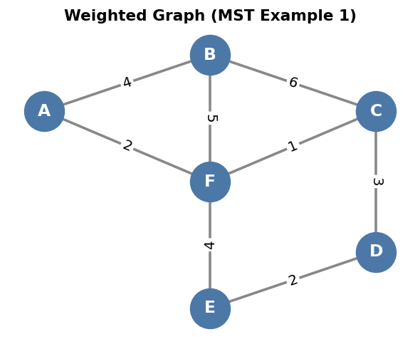
Sorted edges: C-F(1), A-F(2), D-E(2), C-D(3), A-B(4), E-F(4), B-F(5), B-C(6)
| Edge | Weight | Endpoints in same set? | Decision |
|---|---|---|---|
| C-F | 1 | No | Add |
| A-F | 2 | No | Add |
| D-E | 2 | No | Add |
| C-D | 3 | No (joins {A,C,F} & {D,E}) | Add |
| A-B | 4 | No | Add (5 edges → stop) |
| E-F | 4 | Yes | Skip (cycle) |
MST edges: C-F(1), A-F(2), D-E(2), C-D(3), A-B(4) · Total weight = 1+2+2+3+4 = 12
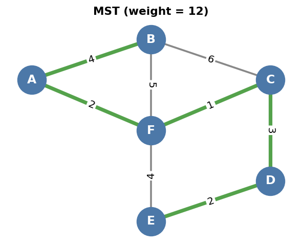
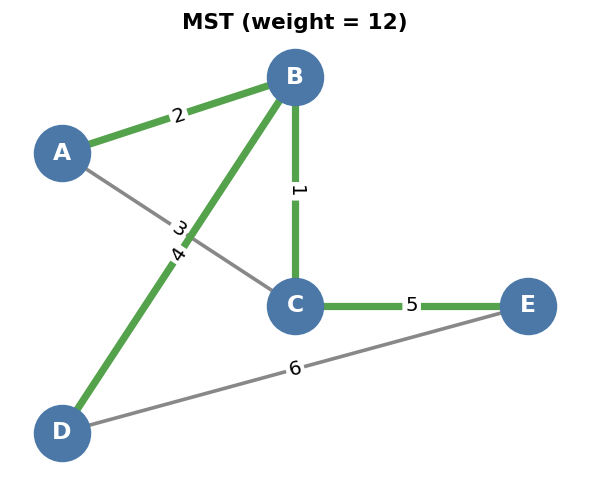
Example 2 — Kruskal on a second graph (V = 5)
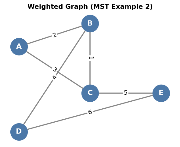
Sorted edges: B-C(1), A-B(2), A-C(3), B-D(4), C-E(5), D-E(6)
| Edge | Weight | Same set? | Decision |
|---|---|---|---|
| B-C | 1 | No | Add |
| A-B | 2 | No | Add |
| A-C | 3 | Yes (A,C connected) | Skip (cycle) |
| B-D | 4 | No | Add |
| C-E | 5 | No | Add (4 edges → stop) |
MST edges: B-C(1), A-B(2), B-D(4), C-E(5) · Total weight = 12
Java Code (with Union–Find)
import java.util.*;

public class Kruskal {
    static int[] parent;

    static int find(int x) {                     // with path compression
        return parent[x] == x ? x : (parent[x] = find(parent[x]));
    }
    static void union(int a, int b) { parent[find(a)] = find(b); }

    public static void main(String[] args) {
        int V = 6;   // A=0, B=1, C=2, D=3, E=4, F=5
        int[][] edges = {
            {2,5,1},{0,5,2},{3,4,2},{2,3,3},{0,1,4},{4,5,4},{1,5,5},{1,2,6}
        };
        Arrays.sort(edges, (x, y) -> x[2] - y[2]);   // sort by weight

        parent = new int[V];
        for (int i = 0; i < V; i++) parent[i] = i;

        int total = 0, count = 0;
        for (int[] e : edges) {
            if (find(e[0]) != find(e[1])) {          // no cycle
                union(e[0], e[1]);
                total += e[2]; count++;
                System.out.println("Edge " + e[0] + "-" + e[1] + "  w=" + e[2]);
                if (count == V - 1) break;
            }
        }
        System.out.println("MST total weight = " + total);   // 12
    }
}
Complexity: O(E log E) — dominated by sorting the edges. Best for sparse graphs.
9.6.2 Prim's Algorithm
Concept (detailed)
Prim's algorithm is vertex-based and greedy. It grows the MST from a single starting vertex, repeatedly adding the minimum-weight edge that connects a vertex already in the MST to a vertex not yet in the MST. Unlike Kruskal, Prim always keeps one connected tree that grows one vertex at a time until all vertices are included.
Pseudocode
procedure PRIM(G, start)
    MST ← empty set
    add start to the "in-tree" set
    while not all vertices are in the tree do
        find the minimum-weight edge (u, v)
              where u is in the tree and v is NOT in the tree
        add v to the tree and add edge (u, v) to MST
    end while
    return MST
end procedure
Algorithm (step form)
- Start from any vertex; mark it as "in the tree."
- Look at all edges that cross from the tree to outside vertices.
- Choose the crossing edge with the smallest weight; add its outside vertex and the edge to the MST.
- Repeat until every vertex is in the tree (V − 1 edges added).
Example 1 — Prim on the same graph as MST Example 1, starting from A
| Step | Tree vertices | Candidate crossing edges | Chosen (min) |
|---|---|---|---|
| 1 | {A} | A-B(4), A-F(2) | A-F (2) |
| 2 | {A, F} | A-B(4), F-C(1), F-B(5), F-E(4) | F-C (1) |
| 3 | {A, C, F} | A-B(4), F-B(5), F-E(4), C-B(6), C-D(3) | C-D (3) |
| 4 | {A, C, D, F} | A-B(4), F-B(5), F-E(4), C-B(6), D-E(2) | D-E (2) |
| 5 | {A, C, D, E, F} | A-B(4), F-B(5), C-B(6) | A-B (4) |
MST edges: A-F(2), F-C(1), C-D(3), D-E(2), A-B(4) · Total weight = 12 (same MST as Kruskal).
Example 2 — Prim on MST Example 2, starting from A
| Step | Tree vertices | Candidate crossing edges | Chosen (min) |
|---|---|---|---|
| 1 | {A} | A-B(2), A-C(3) | A-B (2) |
| 2 | {A, B} | A-C(3), B-C(1), B-D(4) | B-C (1) |
| 3 | {A, B, C} | B-D(4), C-E(5) | B-D (4) |
| 4 | {A, B, C, D} | C-E(5), D-E(6) | C-E (5) |
MST edges: A-B(2), B-C(1), B-D(4), C-E(5) · Total weight = 12
Java Code (O(V²) version with a key array)
import java.util.*;

public class Prim {
    public static void main(String[] args) {
        int V = 6, INF = Integer.MAX_VALUE;
        // A=0,B=1,C=2,D=3,E=4,F=5 ; 0 means no edge
        int[][] g = {
            //  A   B   C   D   E   F
            {   0,  4,  0,  0,  0,  2 },  // A
            {   4,  0,  6,  0,  0,  5 },  // B
            {   0,  6,  0,  3,  0,  1 },  // C
            {   0,  0,  3,  0,  2,  0 },  // D
            {   0,  0,  0,  2,  0,  4 },  // E
            {   2,  5,  1,  0,  4,  0 }   // F
        };
        boolean[] inMST = new boolean[V];
        int[] key = new int[V];
        Arrays.fill(key, INF);
        key[0] = 0;
        int total = 0;

        for (int c = 0; c < V; c++) {
            int u = -1;
            for (int i = 0; i < V; i++)                 // pick min key not in MST
                if (!inMST[i] && (u == -1 || key[i] < key[u])) u = i;
            inMST[u] = true;
            total += key[u];
            for (int v = 0; v < V; v++)                 // update neighbours
                if (g[u][v] != 0 && !inMST[v] && g[u][v] < key[v])
                    key[v] = g[u][v];
        }
        System.out.println("MST total weight = " + total);   // 12
    }
}
Complexity: O(V²) with an adjacency matrix, or O(E log V) with a min-heap. Best for dense graphs.
Kruskal vs Prim
| Feature | Kruskal | Prim |
|---|---|---|
| Approach | Edge-based | Vertex-based |
| Data structure | Sorted edges + Union-Find | Priority queue / key array |
| Grows | A forest that merges into one tree | One tree from a start vertex |
| Best for | Sparse graphs | Dense graphs |
| Complexity | O(E log E) | O(E log V) / O(V²) |
9.7 Shortest Path Problem — Dijkstra's Algorithm
The shortest path problem is finding a path of minimum total weight between vertices in a weighted graph. Dijkstra's algorithm solves the single-source shortest path problem: it finds the shortest distance from one source vertex to all other vertices. It works only when all edge weights are non-negative.
Concept (detailed)
Dijkstra keeps a tentative distance dist[] for every vertex (0 for the source, ∞ for the rest). It repeatedly:
- picks the unfinalized vertex with the smallest tentative distance,
- marks it finalized (its shortest distance is now known), and
- relaxes all its edges — if going through this vertex gives a shorter distance to a neighbour, it updates the neighbour's distance.
Relaxation: if dist[u] + weight(u,v) < dist[v] then dist[v] = dist[u] + weight(u,v).
Pseudocode
procedure DIJKSTRA(G, source)
    for each vertex v do dist[v] ← ∞
    dist[source] ← 0
    put all vertices into a min-priority queue keyed by dist
    while queue is not empty do
        u ← vertex with smallest dist (remove from queue)
        for each neighbour v of u do
            if dist[u] + weight(u, v) < dist[v] then
                dist[v] ← dist[u] + weight(u, v)     // relaxation
            end if
        end for
    end while
    return dist
end procedure
Algorithm (step form)
- Set the source distance to 0 and all others to ∞.
- Select the unvisited vertex with the smallest distance and finalize it.
- For each neighbour, relax the edge (update the neighbour's distance if a shorter route is found).
- Repeat steps 2–3 until all vertices are finalized.
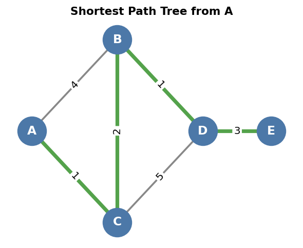
Example 1 — Dijkstra from source A
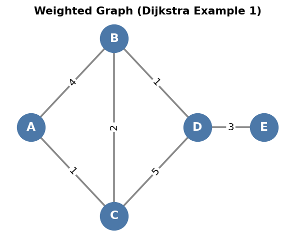
Edges: A-B(4), A-C(1), C-B(2), B-D(1), C-D(5), D-E(3).
| Step | Finalized (picked) | dist A | dist B | dist C | dist D | dist E |
|---|---|---|---|---|---|---|
| init | — | 0 | ∞ | ∞ | ∞ | ∞ |
| 1 | A (0) | 0 | 4 | 1 | ∞ | ∞ |
| 2 | C (1) | 0 | 3 | 1 | 6 | ∞ |
| 3 | B (3) | 0 | 3 | 1 | 4 | ∞ |
| 4 | D (4) | 0 | 3 | 1 | 4 | 7 |
| 5 | E (7) | 0 | 3 | 1 | 4 | 7 |
Shortest distances from A: A=0, B=3, C=1, D=4, E=7. Shortest paths: A→C (1); A→C→B (3); A→C→B→D (4); A→C→B→D→E (7).
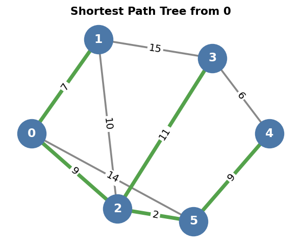
Example 2 — Dijkstra from source 0 (classic 6-vertex graph)
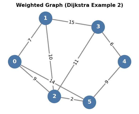
Edges: 0-1(7), 0-2(9), 0-5(14), 1-2(10), 1-3(15), 2-3(11), 2-5(2), 3-4(6), 4-5(9).
| Step | Picked | d0 | d1 | d2 | d3 | d4 | d5 |
|---|---|---|---|---|---|---|---|
| init | — | 0 | ∞ | ∞ | ∞ | ∞ | ∞ |
| 1 | 0 (0) | 0 | 7 | 9 | ∞ | ∞ | 14 |
| 2 | 1 (7) | 0 | 7 | 9 | 22 | ∞ | 14 |
| 3 | 2 (9) | 0 | 7 | 9 | 20 | ∞ | 11 |
| 4 | 5 (11) | 0 | 7 | 9 | 20 | 20 | 11 |
| 5 | 3 (20) | 0 | 7 | 9 | 20 | 20 | 11 |
| 6 | 4 (20) | 0 | 7 | 9 | 20 | 20 | 11 |
Shortest distances from 0: 0=0, 1=7, 2=9, 3=20, 4=20, 5=11. Sample paths: 0→2→5 (11); 0→2→3 (20); 0→2→5→4 (20).
Java Code (min-heap / PriorityQueue)
import java.util.*;

public class Dijkstra {
    public static void main(String[] args) {
        int V = 5;               // A=0,B=1,C=2,D=3,E=4
        List<List<int[]>> adj = new ArrayList<>();
        for (int i = 0; i < V; i++) adj.add(new ArrayList<>());
        addEdge(adj, 0, 1, 4); addEdge(adj, 0, 2, 1); addEdge(adj, 2, 1, 2);
        addEdge(adj, 1, 3, 1); addEdge(adj, 2, 3, 5); addEdge(adj, 3, 4, 3);

        int[] dist = new int[V];
        Arrays.fill(dist, Integer.MAX_VALUE);
        dist[0] = 0;

        // min-priority queue of {vertex, distance}
        PriorityQueue<int[]> pq = new PriorityQueue<>((a, b) -> a[1] - b[1]);
        pq.add(new int[]{0, 0});

        while (!pq.isEmpty()) {
            int[] cur = pq.poll();
            int u = cur[0], d = cur[1];
            if (d > dist[u]) continue;                 // stale entry
            for (int[] e : adj.get(u)) {               // relaxation
                int v = e[0], w = e[1];
                if (dist[u] + w < dist[v]) {
                    dist[v] = dist[u] + w;
                    pq.add(new int[]{v, dist[v]});
                }
            }
        }
        System.out.println(Arrays.toString(dist));     // [0, 3, 1, 4, 7]
    }

    static void addEdge(List<List<int[]>> adj, int u, int v, int w) {
        adj.get(u).add(new int[]{v, w});
        adj.get(v).add(new int[]{u, w});               // undirected
    }
}
Complexity: O((V + E) log V) with a binary min-heap.
9.8 Applications of Graph
- Maps & GPS navigation — cities as vertices, roads as weighted edges; Dijkstra finds the shortest route.
- Social networks — people as vertices, friendships/follows as edges; used for friend suggestions.
- Computer networks — routers/computers as vertices; routing protocols find efficient paths.
- Web & search engines — web pages as vertices, hyperlinks as directed edges (PageRank).
- Network/utility design — laying cables, pipelines, or roads at minimum cost (MST via Kruskal/Prim).
- Task scheduling — dependencies modeled as a Directed Acyclic Graph (topological sort).
- AI & games — maps/mazes as graphs; BFS/DFS/A* for pathfinding.
- Recommendation systems — users and items as a bipartite graph.
Important Questions with Full Answers
Short Questions (2 marks each)
Q1. Define a graph. How is it different from a tree? A graph is a non-linear data structure consisting of a set of vertices and a set of edges connecting them, written as G = (V, E). Unlike a tree, a graph may contain cycles, need not be connected, has no root or parent–child hierarchy, and a vertex may be connected to any number of other vertices.
Q2. Differentiate between a directed and an undirected graph. In a directed graph, each edge has a direction (an edge A→B allows movement from A to B only, so (A,B) ≠ (B,A)). In an undirected graph, edges have no direction and allow movement both ways, so (A,B) = (B,A). Directed-graph vertices have separate in-degree and out-degree.
Q3. What is a spanning tree? A spanning tree of a connected graph is a subgraph that includes all the vertices, is connected and acyclic (a tree), and contains exactly V − 1 edges.
Q4. State the data structures used by BFS and DFS. BFS uses a queue (FIFO) to visit vertices level by level; DFS uses a stack — either an explicit stack or the recursion call stack — to go as deep as possible before backtracking.
Q5. When is an adjacency list preferred over an adjacency matrix? An adjacency list is preferred for sparse graphs (few edges), because it uses O(V + E) space compared with the adjacency matrix's O(V²), and it lets us iterate a vertex's neighbours in O(degree) time.
Q6. What condition must hold for Dijkstra's algorithm to work correctly? All edge weights must be non-negative. With negative weights, a finalized vertex's distance could later be improved, which Dijkstra does not reconsider, giving wrong results.
Q7. Differentiate between Prim's and Kruskal's approach in one line each. Prim's algorithm grows a single tree by repeatedly adding the cheapest edge from the tree to a new vertex, while Kruskal's algorithm adds the globally cheapest edges one by one (skipping cycles) until all vertices are connected.
Q8. What is the degree of a vertex? The degree of a vertex is the number of edges connected to (incident on) it. In a directed graph, it is split into in-degree (incoming edges) and out-degree (outgoing edges).
Long Questions (6 marks each)
Q1. Explain BFS and DFS with algorithms, a traced example, and a comparison.
BFS (Breadth-First Search) visits a graph level by level using a queue: it marks the start visited, enqueues it, then repeatedly dequeues a vertex, visits it, and enqueues all its unvisited neighbours. DFS (Depth-First Search) goes as deep as possible using recursion/stack: it visits a vertex, then recursively visits an unvisited neighbour, backtracking when a dead end is reached.
Trace on graph G1 (0→[1,2], 1→[0,3,4], 2→[0,4], 3→[1,5], 4→[1,2,5], 5→[3,4]) from vertex 0:
- BFS: dequeue 0 (add 1,2), dequeue 1 (add 3,4), dequeue 2, dequeue 3 (add 5), dequeue 4, dequeue 5 → order 0 1 2 3 4 5.
- DFS: 0→1→3→5→4→2 → order 0 1 3 5 4 2.
Comparison: BFS uses a queue, explores widely, and finds the shortest path in unweighted graphs but needs more memory; DFS uses a stack/recursion, explores deeply, uses less memory, and is used for cycle detection, topological sorting, and maze solving. Both run in O(V + E).
Q2. Explain the two graph representation methods with examples and state the advantages of each.
A graph can be represented using an adjacency matrix or an adjacency list. The adjacency matrix is a V×V array where entry [i][j] is 1 (or the weight) if an edge exists between i and j, else 0; for undirected graphs it is symmetric. It allows O(1) edge lookup but uses O(V²) space, making it suitable for dense graphs. The adjacency list stores, for each vertex, a list of its neighbours; it uses O(V + E) space and lets us iterate neighbours in O(degree) time, making it ideal for sparse graphs (most real-world graphs). For the graph with edges {0-1, 0-2, 1-2, 2-3}, the matrix has 1s at those positions, while the list is 0→[1,2], 1→[0,2], 2→[0,1,3], 3→[2].
Q3. What is a Minimum Spanning Tree? Explain Kruskal's algorithm with a complete solved example.
A Minimum Spanning Tree (MST) of a weighted connected graph is a spanning tree (all vertices, V−1 edges, no cycle) whose total edge weight is the minimum possible. Kruskal's algorithm is a greedy, edge-based method: sort all edges in ascending weight order, then add each edge to the MST if it does not form a cycle (checked with Union–Find), stopping at V−1 edges.
Solved example (V=6): edges sorted are C-F(1), A-F(2), D-E(2), C-D(3), A-B(4), E-F(4), B-F(5), B-C(6). Adding C-F, A-F, D-E, C-D, and A-B gives 5 edges with no cycles (E-F is skipped because it would form a cycle). The MST edges are C-F(1), A-F(2), D-E(2), C-D(3), A-B(4) with total weight 12. Kruskal's complexity is O(E log E), dominated by sorting.
Q4. Explain Prim's algorithm with a solved example, and compare it with Kruskal's algorithm.
Prim's algorithm is a greedy, vertex-based MST method. Starting from any vertex, it repeatedly adds the minimum-weight edge that connects a vertex already in the tree to a vertex outside it, until all vertices are included.
Solved example (V=6, start A): choose A-F(2), then F-C(1), then C-D(3), then D-E(2), then A-B(4). MST edges: A-F(2), F-C(1), C-D(3), D-E(2), A-B(4), total weight 12 — the same MST Kruskal produces.
Comparison: Prim is vertex-based and grows one connected tree using a priority queue/key array (good for dense graphs, O(E log V) or O(V²)); Kruskal is edge-based, sorts all edges, and uses Union–Find to merge components (good for sparse graphs, O(E log E)). Both are greedy and produce an MST of the same total weight.
Long Questions (10 marks each)
Q1. Explain Dijkstra's algorithm for the single-source shortest path with pseudocode, a fully solved traced example, and its complexity. State one limitation.
Dijkstra's algorithm finds the shortest distance from a single source to all other vertices in a graph with non-negative edge weights. It maintains a tentative distance array (0 for the source, ∞ for others). Repeatedly, it picks the unfinalized vertex with the smallest distance, finalizes it, and relaxes each outgoing edge: if dist[u] + weight(u,v) < dist[v], it updates dist[v].
Pseudocode: initialize dist[source]=0 and the rest to ∞; put all vertices in a min-priority queue; while the queue is not empty, extract the vertex u with the smallest distance and relax all its neighbours.
Solved trace from source A on edges A-B(4), A-C(1), C-B(2), B-D(1), C-D(5), D-E(3):
- Pick A(0): B=4, C=1.
- Pick C(1): B=min(4, 1+2)=3, D=min(∞, 1+5)=6.
- Pick B(3): D=min(6, 3+1)=4.
- Pick D(4): E=4+3=7.
- Pick E(7): done. Final shortest distances: A=0, C=1, B=3, D=4, E=7, with paths such as A→C→B→D→E for E.
Complexity: O((V + E) log V) using a binary min-heap. Limitation: it fails with negative edge weights, because once a vertex is finalized Dijkstra never revisits it, so a later cheaper path through a negative edge would be missed (the Bellman–Ford algorithm handles negative weights).
Q2. Describe graphs completely: definition, terminology, types, representation, and any four real-world applications. Support with diagrams/examples.
A graph G = (V, E) is a non-linear structure of vertices connected by edges, able to contain cycles and multiple connections per vertex. Key terminology includes vertex, edge, adjacent vertices, degree (in-degree/out-degree for directed graphs), path, cycle, weighted edge, connected graph, and spanning tree.
Types of graphs: an undirected graph has two-way edges where (A,B) = (B,A) (e.g., friendship); a directed graph has one-way edges where (A,B) ≠ (B,A) (e.g., web links). Additional types include weighted vs unweighted, cyclic vs acyclic (a DAG is a directed acyclic graph), and connected vs disconnected.
Representation: graphs are stored as an adjacency matrix (V×V array; O(1) edge lookup but O(V²) space, good for dense graphs) or an adjacency list (list of neighbours per vertex; O(V + E) space, good for sparse graphs). For edges {0-1, 0-2, 1-2, 2-3}, the adjacency list is 0→[1,2], 1→[0,2], 2→[0,1,3], 3→[2].
Four applications: (1) GPS/maps use weighted graphs with Dijkstra for shortest routes; (2) social networks model people and friendships for recommendations; (3) utility/network design uses MST algorithms (Kruskal/Prim) to connect all points at minimum cost; (4) task scheduling uses directed acyclic graphs with topological sorting to order dependent tasks. Other uses include web ranking, computer-network routing, and AI pathfinding in games.
Lab Questions
Write a Java program to represent a graph using an adjacency list or adjacency matrix and implement Breadth-First Search (BFS) and Depth-First Search (DFS) traversal algorithms.
Write a Java program to implement Kruskal's algorithm, Prim's algorithm, and Dijkstra's algorithm for finding the Minimum Spanning Tree (MST) and the shortest path in a weighted graph.
End of Unit IX — Graph.